Quick Overview on LLM Serving and Benchmarking
/ 25 min read
Introduction
Before you dive into LLM application development, let’s first address how to serve these powerful language models effectively.
Over the past nine months, my experience with deploying Large Language Models (LLMs) has been both challenging and enlightening. As part of a team dedicated to developing an LLM platform and managing its operations, I’ve worked to introduce the latest advancements in the field to internal users within the company. During this time, the LLM landscape has evolved rapidly, with frontier labs frequently releasing more advanced models. While the initial craze began with OpenAI’s ChatGPT, today’s closed-source LLMs such as GPT-4, Claude 3 Opus, and Gemini Ultra should no longer be seen as the default choices for business use cases. This shift is due to the emergence of increasingly capable open-source models like Llama 3, Mistral (and Mixtral).
Why is this change significant? Dealing with compliance and potential data security issues, especially regarding internal data leaks, can be a major headache (though enterprise offerings have improved in this regard). Additionally, it is still challenging to fully integrate meaningful enterprise data with these LLMs despite their purported capabilities. From an enterprise perspective, there’s much room for improvement (no more chatbots, please!).
Although proprietary LLMs are currently more capable than open-source models, the flexibility of open-source models offers greater potential for improvement beyond simply augmenting closed-source LLMs with techniques such as RAG.
Therefore, open-source LLMs remain highly relevant within enterprise settings due to factors like cost and customizability (e.g., fine-tuning). Consequently, a key aspect of my job involves deploying the latest open-source models for exploration and productionisation.
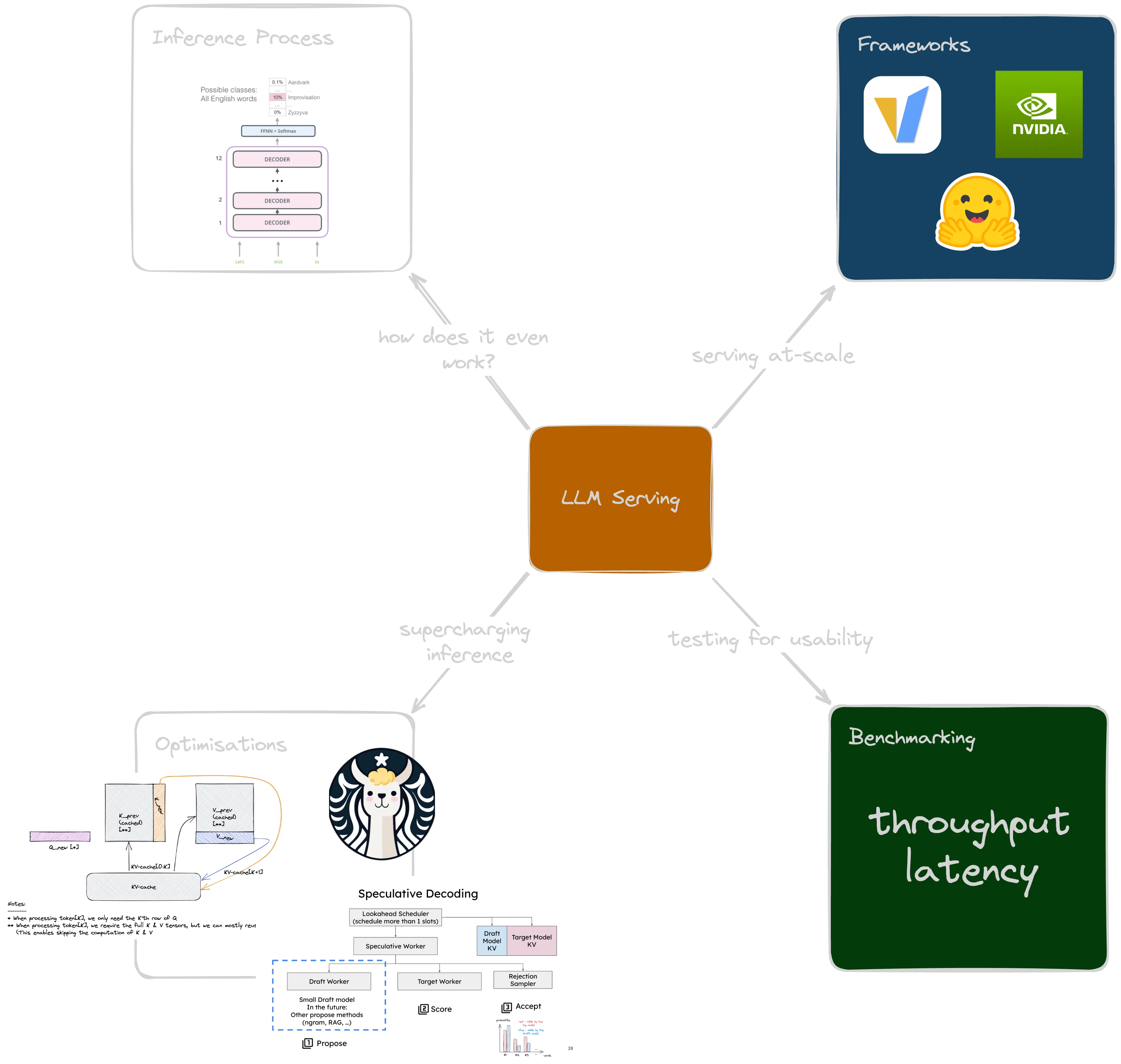
In this post, I cover some of my learnings on:
- How LLM inference works, as well as the latest advancement in optimizing LLM serving at-scale
- Common LLM serving frameworks
- Benchmarking performance of LLM deployments
Key Fundamentals
Before moving into the various aspects of LLM serving, let’s first explore some fundamental concepts behind LLM inference and areas of optimization.
These foundational ideas are crucial in enhancing the performance and efficiency of popular serving frameworks that I personally use at work.
LLM Inference Process
Understanding LLM inference is a prerequisite to efficiently serve a model.
While the topic here is about LLM serving, it’s crucial to first understand how LLM inference works. Broadly, the inference process can be divided into two separate phases:
- Input Encoding: This phase involves tokenizing the user’s input, converting it into embeddings, and passing these through the LLM architecture (typically based on Transformers).
The input encoding process is also known as the prefill phase, during which the LLM computes the
intermediate state of the Key-Value (KV) cache (we’ll discuss the KV cache in more detail later).
- Output Decoding: In this phase, the model generates the next token in the sequence in an autoregressive manner.
The output decoding process usually reiterates until a stopping criterion is met. Examples of stopping criteria include reaching the maximum token limit or encountering a specific stop token, such as Mistral 7B’s </s>.
More on the inference process here.
Areas of Optimisation
Due to the auto-regressive nature of models like GPT-4, inference can be relatively slow. For instance, to generate a short 10-word sentence, the model must produce each word sequentially, one after the other.
Additionally, the sheer size of models such as GPT-4 and Claude-3 Opus, with their billions of parameters, demands substantial computational resources. This often leads to memory bandwidth constraints, where the time taken to read from and write to memory becomes a significant overhead and a bottleneck in the inference process.
However, there have been some initial and more recent advancements aimed at optimizing the inference process.
KV Cache
Trading Memory for Compute.
I briefly mentioned the KV cache in the input encoding (or prefill) phase, but what exactly does a KV cache do? In simple terms, a KV cache stores the keys and values generated from previous words (tokens) during the prediction of the next word within a sentence. This is crucial considering that the attention mechanism in vanilla Transformers is quadratic in nature, leading to increased computational demands as the sequence length grows.
The KV cache is first utilized during the prefill phase, where intermediate states are computed for each token within the input sequence. This phase sets up the essential information required for the KV cache’s true utilization in the decoding (generation) phase. During decoding, the LLM refers to the stored keys and values from the input sequence within the KV cache to predict the next token.
By leveraging the KV cache, we avoid reprocessing every prior token’s information at each step when generating a new token. Instead, we only use the information from the last generated token stored within the KV cache, effectively reducing the computation requirements of the attention mechanism to a linear complexity. However, this efficiency comes at the cost of higher memory usage.
While diving deeply into the trade-offs of KV caching is beyond our current scope, you can explore further here.
Beside KV cache, we should also consider common optimizations that help manage increased memory usage, as reduced memory usage means fewer GPUs are required to serve a LLM.
PagedAttention
Inspired by Virtual Memory and Paging in operating systems.
One advancement made to the attention mechanism that improves LLM serving is PagedAttention.
Initially developed by the team behind vLLM, PagedAttention has now been integrated behind other popular serving frameworks such as TGI, TensorRT-LLM, etc.
It addresses memory wastage issues in existing KV cache setups (in particular, attention keys and values) by tackling several key problems:
- Internal Fragmentation: Over-allocating memory due to unknown output length.
- Reservation: Allocated memory not used at the current step but required in the future.
- External Fragmentation: Memory inefficiency due to varying sequence lengths.
PagedAttention mitigates these issues by storing continuous keys and values in non-contiguous memory blocks of fixed size. This approach significantly improves memory utilization, with claims of a 3-5x enhancement. Specifically, less than 4% of the KV cache space is wasted, as internal fragmentation occurs only within the last block of the sequence.
Furthermore, PagedAttention enables memory sharing during the decoding phase, allowing multiple output sequences to be generated from the same input sequence. This reduces memory overhead from complex sampling algorithms such as parallel sampling and beam search.
But how do these memory optimizations improve LLM inference? It all comes down to:
- Reduced Memory Wastage: By minimizing memory wastage compared to traditional KV cache methods, you can handle more requests simultaneously, thereby increasing overall throughput.
- Sharing Computations: The ability to share prior computations when similar prefix sequences are encountered further boosts throughput due to reduced memory usage.
For a more detailed understanding, you can refer to the official paper 1.
Batching
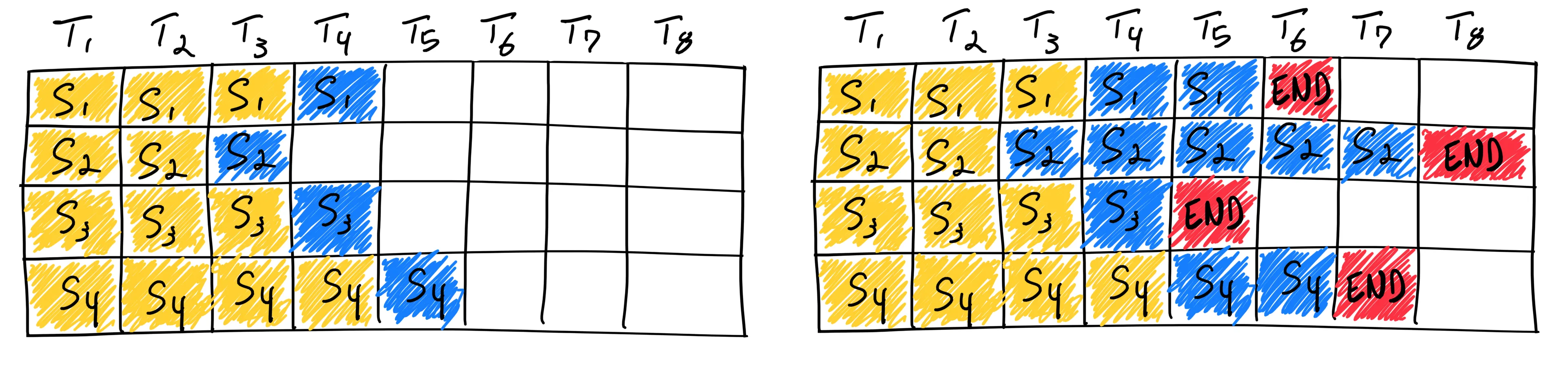
Illustration of static vs continuous batching by
Anyscale
.
The LLM inference process is memory-bound, involving frequent read and write operations to memory without maximizing the potential of the GPUs’ compute power. This inefficiency in resource utilization can significantly hinder overall performance. One way to address this issue is by increasing the number of sequences processed per iteration of loading model parameters, thereby improving overall computation utilization.
The naive, or more commonly referred to as static batching method, involves sending a fixed batch size of input sequences for inference. However, due to the nature of how LLMs are utilized and behave, not all input sequences processed complete at the same time. This means that even if compute power is available to process additional sequences, it cannot be released for new requests as other sequences are still in the processing stage.
This challenge can be better illustrated with an example. Consider a batch size of 32 sequences, where more than three-quarters of the sequences output only 100 tokens, while the remaining quarter may output 500 or more tokens. This scenario leads to a situation where large amounts of resources remain unutilized because the time to output 100 tokens is much faster. As a result, resources cannot be released for further processing, as they are waiting for the quarter of longer sequences to be completed. This can be further illustrated graphically by the left side of the image above.
A newer approach that has emerged in the industry attempts to fix this inefficiency. Instead of having to wait for the longer sequences to finish, continuous batching continuously schedules new requests as soon as a prior request (sequence) is completed. This method ensures better utilization of available compute power and is further illustrated on the right side of the image above.
Continuous batching allows for better overall throughput and latency, especially in the case of online serving where typically, we would not want users to wait long for the LLM output. The ability to handle requests one after the other without the need to wait for all previously batched requests to complete is crucial to ensure minimal waiting time for each request.
You may also have seen/heard the term in-flight batching, which also refers to continuous batching.
Speculative Decoding
Speculative decoding is an advanced technique designed to accelerate the inference process and reduce token latency in auto-regressive models.
This approach can be better understood by imagining a smaller (draft) model assisting your LLM.
While the smaller model might not be as capable, it can swiftly identify candidate tokens, which the larger model then considers.
Even without using a smaller model, you can leverage your prompt to generate “choices” for your LLM in scenarios where less creative results are needed, such as summarization, by using n-grams – a statistical method for predicting the next token based on previous tokens.
Draft Model
To avoid leaving compute resources idle — since the inference process is often memory-bound — we can utilize a smaller draft model to predict several potential token choices in parallel with the larger model’s inference process. Because smaller models can perform the forward pass faster during inference compared to larger models, they can effectively provide token choices for the larger model to evaluate. To implement this technique, you need to identify a smaller version of the large model that uses the same tokenizer to ensure consistency in token representation and smooth integration of predictions.
For example, to speed up the inference of a model like meta-llama/Llama-2-7b-hf, you might use a smaller model such as JackFram/llama-68m for speculative sampling of tokens, as both share the same tokenizer, as demonstrated in relevant research 2.
However, if the size difference between the draft and the target models is too significant, the output quality may suffer.
Therefore, if computational resources allow, consider using a larger draft model to minimize this size disparity.
For instance, you could use facebook/opt-1.3b alongside facebook/opt-6.7b to ensure more consistent results.
N-gram
An alternative approach to speculative decoding with a smaller draft model is employing the n-gram method in context-dependent tasks. Tasks such as summarization, document QA, and code editing often exhibit high n-gram overlap, meaning the generated text by the LLM tends to match sequences of tokens in the original input or prompt.
By leveraging these potential matches, we can assist the LLM in making token considerations. Specifically, we can derive n-grams from the prompt to generate potential token candidates, which the LLM can then evaluate and incorporate into the generated output.
Similar to the draft model approach, this method requires no modification to the model itself, yet can achieve significant speed-ups in scenarios where outputs and inputs share similar token sequences.
MEDUSA
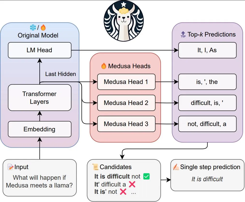
MEDUSA pipeline from the official GitHub repository.
Speculative decoding methods like the draft model and n-grams involve no modification to the existing LLM. In contrast, MEDUSA adopts a different approach by adding additional “heads” to the LLM in a parameter-efficient 3 manner.
The creators of MEDUSA identified key issues with traditional speculative decoding methods, such as the challenge of finding a good draft model and the overall system complexity of deploying an additional model for generating token candidates.
In MEDUSA, the additional “heads” are trained decoder heads added to the model that is being used. This method is parameter-efficient because, in the initial approach (MEDUSA-1), only the new decoder heads are trained while the base model remains frozen.
The latest version (MEDUSA-2), however, includes full-model training, which results in even greater speedup. According to the paper 4, MEDUSA can achieve a speedup of 2.2-2.8x 5 times across different prompts without compromising quality.
MEDUSA’s core idea involves using the newly trained decoder heads to predict tokens. Specifically, the k-th head predicts a token for the timestamp at the -th position, whereas the original LLM decoder head predicts only the -th position. Essentially, MEDUSA attempts to predict tokens for multiple timesteps from the next token position. If token candidates are selected based on custom acceptance criteria (extended from those used in the draft model), MEDUSA can bypass several forward passes required by the LLM to generate the selected tokens, using the outputs from the newly added decoder heads.
In addition to the decoder heads, MEDUSA uses tree attention — a tree-structured attention mechanism — where only predecessor tokens are used as tokens for the attention flow. This involves employing a custom tree-structure attention mask.
If you’re interested in more in-depth explanations of the various speculative decoding techniques, Julien Simon from HuggingFace provides excellent insights on how each technique works
Overview on various LLM inference optimisation techniques by
Julien Simon
.
Components of LLM Serving
Now that we’ve covered the basics of LLM inference and explored optimization techniques, let’s move on to the topic of LLM serving.
The folks at Run:ai have written a similar article that covers the journey from LLM inference to serving and also provided a concise architecture diagram illustrating what LLM serving should look like:
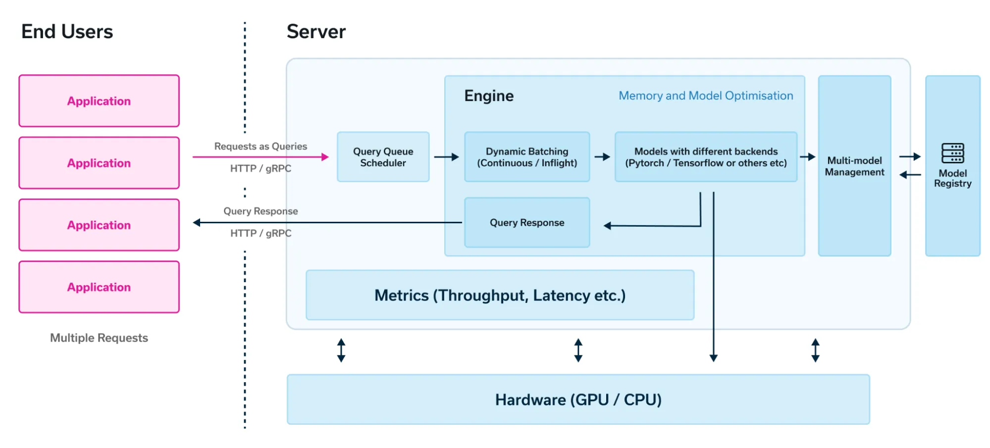
While there are some distinctions made when serving LLMs, such as:
- Engines: Load and runs the model
- Servers: Orchestrating user HTTP/gPRC requests
In practice, serving frameworks typically satisfy both aspects. For example, vLLM, as an inference engine, also provides an OpenAI-compatible HTTP server built with FastAPI.
However, we should still evaluate serving frameworks based on the following capabilities:
- Memory management of KV cache
- Memory optimisation
- Model specific optimisation
- Batch support
- HTTP/gRPC API support (OpenAI API compatibility allows for greater flexibility in integrating with existing LLM applications)
- Request queuing
Established Frameworks
Keeping the previously mentioned capabilities in mind, let’s take a deeper look into some of the most popular serving frameworks available today.
vLLM

vLLM has rapidly emerged as the go-to open-source framework for serving large language models (LLMs), cementing its popularity among developers. Boasting an impressive 21.9k stars on GitHub, vLLM is a top choice for those looking to deploy LLMs at scale.
Developed at UC Berkeley, vLLM is renowned for popularizing the innovative PagedAttention technique, which has since been adopted by other frameworks like TGI and TensorRT-LLM. As of now, vLLM supports up to 38 distinct transformer architectures. This versatility allows developers to deploy dozens or even hundreds of different LLMs using a single, streamlined workflow.
Notable Features and Capabilities
-
Efficient memory management with PagedAttention
- Pioneering the use of PagedAttention for enhanced memory efficiency, allowing for the deployment of larger models with less resource overhead.
-
Continuous batching of inference requests
- Dynamically batches incoming requests to maximize throughput and minimize latency, ensuring efficient utilization of resources.
-
Fast model execution with CUDA/HIP graph
- Utilizes CUDA and HIP graph technologies to accelerate model execution, providing faster inference times.
-
Support for a wide range of GPUs and accelerators
- Compatible with hardware from NVIDIA and AMD, as well as cloud-based options like AWS Trainium and GCP TPUs, offering flexibility in deployment environments.
-
Optimized CUDA kernels
- Features highly optimized CUDA kernels for high performance on NVIDIA GPUs.
-
Distributed inference with tensor parallelism
- Enables parallelism across multiple GPUs for distributed inference, scaling up performance and efficiency.
-
OpenAI-compatible API server
- Features an API server compatible with OpenAI’s API, making it easier to switch between frameworks without changing client-side code.
-
Support for Multimodal Model
- Includes ability to serve Large Multimodal Models such as LlaVA.
-
Support for Multi-nodes with Ray
- Leverages Ray for multi-node support, enabling distributed LLM serving across multiple nodes to handle larger complex models efficiently.
-
Production-Ready Inference Server with OpenTelemetry Tracing and Prometheus Metrics
- Offers a robust, production-ready inference server that integrates with OpenTelemetry and Prometheus, enabling comprehensive observability and monitoring.
Some other features still in experimental stage (yet to be optimised as per documentation) includes:
- Prefix caching
- Multi-LoRA support
- Speculative decoding methods such as draft model and n-grams etc.
TensorRT-LLM
From NVIDIA, TensorRT-LLM stands out as a popular alternative to vLLM for serving large language models (LLMs), offering seamless integration with the NVIDIA Triton Inference Server.
With a strong following of 7.4k stars on GitHub, TensorRT-LLM supports approximately 40+ different transformer architectures, making it a robust choice for developers looking to leverage NVIDIA’s hardware for high-performance LLM serving.
Notable Features and Capabilities
-
Optimized inference with compiled model via TensorRT
- Utilizes TensorRT for optimized inference by compiling models to run efficiently on NVIDIA GPUs, enhancing both speed and performance.
-
Efficient memory management with PagedAttention
-
Continuous batching of inference requests
-
Distributed inference with tensor and pipeline parallelism
-
Improve token latency with speculative decoding
- Reduce per-token latency with speculative decoding methods such as draft model and MEDUSA.
-
Support for wide range of Multimodal Model
-
Support for Multi-nodes
- Inference on multi-node, multi-GPU setups is achievable using MPI in conjunction with NVIDIA’s NCCL.
TGI
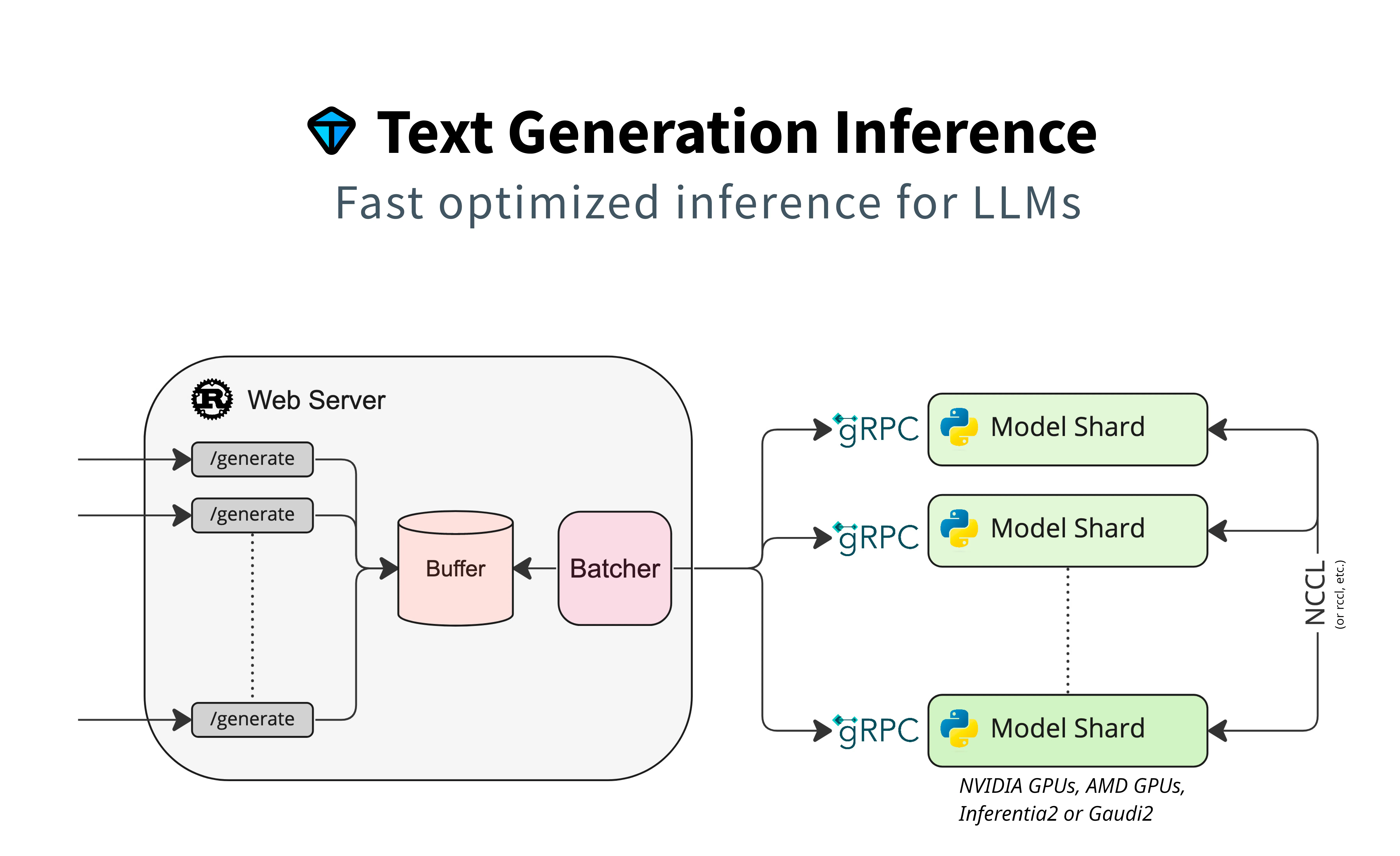
Text Generation Inference (TGI), created by the developers of transformers, is a serving framework that has gained popularity with 8.3k stars on GitHub.
It provides support for approximately 26 different model architectures. With direct integration with the HuggingFace Hub, TGI offers a simple launcher to quickly deploy LLMs on your infrastructure.
Notably, if a specific model architecture is not directly supported, but is available in the transformers library, the deployment will fallback to the default transformers implementation. However, this fallback lacks capabilities in tensor parallelism and flash attention.
Notable Features and Capabilities
-
Efficient memory management with PagedAttention
-
Continuous batching of inference requests
-
Support for a range of GPUs and accelerators
- Compatible with hardware from NVIDIA and AMD, as well as cloud-based options like AWS Inferentia and Intel HPUs (Gaudi), offering flexibility in deployment environments.
-
Distributed inference with tensor parallelism
-
Improve token latency with speculative decoding
- Reduce per-token latency with speculative decoding methods such as draft model, n-grams and MEDUSA.
-
Support for Multimodal Model
-
OpenAI-compatible API server
-
Production-Ready Inference Server with OpenTelemetry Tracing and Prometheus Metrics
Systematic Approach to Benchmarking Performance
User experience is crucial. Make sure to test the performance of your LLM deployments!
Deploying a large language model (LLM) can be relatively straightforward once you have the necessary resources in place, especially if you use the appropriate serving frameworks such as vLLM, TensorRT-LLM etc. The primary considerations involve setting up the right infrastructure and ensuring that your compute hardware can handle the size of the model and deliver the desired performance levels.
However, it is crucial to ensure that the LLM performs well during inference to be considered viable for integration into any production applications. Acceptable performance standards — such as low latency and high throughput — are essential for the effective use of LLMs in real-world scenarios. Monitoring and optimizing these metrics can help maintain performance benchmarks. By addressing these considerations, you can facilitate the integration of LLMs into production systems, ensuring they meet the performance criteria required for practical applications.
Therefore, benchmarking remains a critical aspect of the LLM serving process. To evaluate the serving frameworks, the following metrics are commonly considered:
Throughput
Throughput is a straightforward metric that measures the overall output produced by your deployed LLM. It is often measured in two forms:
-
Request Throughput: How many requests can the system serve in a minute (
req/min)?- You can also consider the number of requests per second (
req/sec).
- You can also consider the number of requests per second (
-
Token Throughput: How many tokens can be produced in a second (
tokens/sec)?
When assessing request throughput, it allows for better understanding of the behavior of the LLM under varying loads, particularly with concurrent requests. This measure depends on the input and output lengths, so one should pay careful attention and possibly use a consistent dynamic dataset when comparing different infrastructures, frameworks, or models.
Alternatively, you can focus on token throughput. Some evaluations include both input and output tokens, but if online inference is the primary concern, focusing on output tokens may make more sense. This approach provides a measure of the “speed” at which the LLM produces tokens.
Latency
Considering the use case for LLM-generated summarization, these tasks are often best suited for batch inference scenarios. In many cases, time is not a critical factor, and users may not have high expectations for immediate results. The primary goal is to generate accurate and comprehensive summaries, which can be batched and processed over longer periods without impacting user satisfaction significantly.
However, this requirement for immediacy changes dramatically in the context of chatbots. In a chatbot scenario, users expect quick and fast responses that mimic real-time interactions they would have with colleagues or support agents. The speed and efficiency of responses are critical for maintaining a satisfactory user experience, particularly when the chatbot is resolving issues or answering queries.
Therefore, while (high) performance latency might be acceptable for summarization tasks, it becomes a crucial metric for chatbot applications. Ensuring low latency in use cases such as chatbot is essential for effective and satisfying user engagement.
This highlights the importance of metrics like Time to First Token and Time per Output Token, which directly impact the perceived responsiveness of interactive applications.
Time to First Token
In streaming use-cases, the Time to First Token (TTFT) is a crucial measure that indicates how long a user will need to wait for the first token to be generated by the inference server and received by the user. This metric is generally not relevant for offline inference scenarios. The primary purpose of TTFT is to understand the processing time for the input prompt until the first generated token is produced.
Monitoring TTFT is essential for optimizing user experience in real-time applications, as it provides insights into the initial latency experienced by the user.
Time per Output Token
Similar to TTFT, Time per Output Token (TPOT) is another measure of latency, but it focuses on the delivery of generated tokens to the user while the LLM is decoding the input prompt. TPOT measures the time taken to generate and deliver each subsequent token after the first one.
TPOT is a critical factor in user experience, as it directly influences whether the user perceives the LLM as fast or slow. Consistent and low TPOT ensures that users experience fluid and responsive interactions, while higher TPOT can make the interaction feel laggy and sluggish. Monitoring and optimizing TPOT is essential for achieving a smooth and efficient user experience in real-time applications.
This post by Databricks further highlights some trade-offs and heuristics involved when looking at the above metrics.
Benchmark Setup
After understanding the key performance metrics when it comes to LLM serving, the question lies – how do you capture these metrics?
Planning
Before you begin running performance benchmarks to capture relevant metrics, the essential first step is to start by planning test scenarios or scopes.
Some points to consider include:
-
Primary Objectives
- Define the goals of measuring performance.
- Determine whether to prioritize latency, throughput-based metrics, or both.
- Assess how the system will manage peak loads and concurrent users.
-
Usage Behaviors and Use Cases
- Identify typical user interactions and queries in a production environment.
- Outline specific use cases for LLM deployments and their performance expectations.
- Evaluate the system’s ability to handle high usage behaviors efficiently, maintaining acceptable latency.
- Analyze the impact of varying input sizes on performance.
By addressing these points, you can effectively plan your benchmarking scenarios to ensure that your performance evaluations are comprehensive and tailored to your specific requirements and use cases.
Furthermore, taking the time to incorporate these considerations will enable you to determine whether your benchmark metrics are truly meeting your objectives. At my current workplace, we initiated benchmarking to assess whether our open-source LLM deployments could adequately support the needs of our use cases.
For example, if the use case demands real-time interaction with the LLM, stakeholders would naturally expect lower latency between the user’s input and the LLM’s output. By benchmarking our deployments, we can provide public figures that help developers understand how each LLM deployment performs. This information is essential for determining whether a particular LLM deployment is suitable for production or whether an alternative needs to be sought.
Execution
The next step post-planning, is to develop the actual benchmarking setup. In my prior work exploration, we found that a straightforward way to get started is to adapt vLLM’s benchmarking scripts to suit your own needs.
For example, let’s refer to the benchmark_serving.py script to understand how we can benchmark online serving throughput.
To start off, we can first define the set of metrics we are keen to capture. In vLLM’s case, they captured the following metrics:
@dataclassclass BenchmarkMetrics: completed: int # no. of completed request total_input: int # no. of input tokens total_output: int # no. of output tokens request_throughput: float # request throughput input_throughput: float # input token throughput output_throughput: float # output token throughput mean_ttft_ms: float # average time to first token median_ttft_ms: float # p50 time to first token p99_ttft_ms: float # p99 time to first token mean_tpot_ms: float # average time per output token median_tpot_ms: float # p50 time per output token p99_tpot_ms: float # p99 time per output token mean_itl_ms: float # average inter-token latency median_itl_ms: float # p50 inter-token latency p99_itl_ms: float # p99 inter-token latencyThe metrics captured consists of measures of throughput and latency-related evaluation. To capture the metrics, dynamic requests are send to the inference endpoint using dataset that consists of actual conversations with LLMs.
def sample_sharegpt_requests(    dataset_path: str,    num_requests: int,    tokenizer: PreTrainedTokenizerBase,    fixed_output_len: Optional[int] = None,) -> List[Tuple[str, int, int]]:    if fixed_output_len is not None and fixed_output_len < 4:        raise ValueError("output_len too small")
    # Load the dataset.    with open(dataset_path) as f:        dataset = json.load(f)    # Filter out the conversations with less than 2 turns.    dataset = [data for data in dataset if len(data["conversations"]) >= 2]    # Only keep the first two turns of each conversation.    dataset = [(data["conversations"][0]["value"],                data["conversations"][1]["value"]) for data in dataset]
    # Shuffle the dataset.    random.shuffle(dataset)
    # Filter out sequences that are too long or too short    filtered_dataset: List[Tuple[str, int, int]] = []    for i in range(len(dataset)):        if len(filtered_dataset) == num_requests:            break
        # Tokenize the prompts and completions.        prompt = dataset[i][0]        prompt_token_ids = tokenizer(prompt).input_ids        completion = dataset[i][1]        completion_token_ids = tokenizer(completion).input_ids        prompt_len = len(prompt_token_ids)        output_len = len(completion_token_ids                         ) if fixed_output_len is None else fixed_output_len        if prompt_len < 4 or output_len < 4:            # Prune too short sequences.            continue        if prompt_len > 1024 or prompt_len + output_len > 2048:            # Prune too long sequences.            continue        filtered_dataset.append((prompt, prompt_len, output_len))
return filtered_datasetDynamic requests refer to requests that not constant throughout the benchmark run, but rather varying in input and output length. This allows us to test the endpoint performance with changing computational complexity.
To ensure that performance is measured in a similar fashion in real-world production settings, asynchronous HTTP client such as aiohttp is used to
send requests asynchronously.
async def async_request_tgi(    request_func_input: RequestFuncInput,    pbar: Optional[tqdm] = None,) -> RequestFuncOutput:    api_url = request_func_input.api_url    assert api_url.endswith("generate_stream")
    async with aiohttp.ClientSession(timeout=AIOHTTP_TIMEOUT) as session:        assert not request_func_input.use_beam_search        params = {            "best_of": request_func_input.best_of,            "max_new_tokens": request_func_input.output_len,            "do_sample": True,            "temperature": 0.01,  # TGI does not accept 0.0 temperature.            "top_p": 0.99,  # TGI does not accept 1.0 top_p.        }        payload = {            "inputs": request_func_input.prompt,            "parameters": params,        }        output = RequestFuncOutput()        output.prompt_len = request_func_input.prompt_len
        ttft = 0.0        st = time.perf_counter()        most_recent_timestamp = st        try:            async with session.post(url=api_url, json=payload) as response:                if response.status == 200:                    async for chunk_bytes in response.content:                        chunk_bytes = chunk_bytes.strip()                        if not chunk_bytes:                            continue                        chunk_bytes = chunk_bytes.decode("utf-8")
                        #NOTE: Sometimes TGI returns a ping response without                        # any data, we should skip it.                        if chunk_bytes.startswith(":"):                            continue                        chunk = remove_prefix(chunk_bytes, "data:")
                        data = json.loads(chunk)                        timestamp = time.perf_counter()                        # First token                        if ttft == 0.0:                            ttft = time.perf_counter() - st                            output.ttft = ttft
                        # Decoding phase                        else:                            output.itl.append(timestamp -                                              most_recent_timestamp)
                        most_recent_timestamp = timestamp
                    output.latency = most_recent_timestamp - st                    output.success = True                    output.generated_text = data["generated_text"]                else:                    output.error = response.reason or ""                    output.success = False        except Exception:            output.success = False            exc_info = sys.exc_info()            output.error = "".join(traceback.format_exception(*exc_info))
        if pbar:            pbar.update(1)        return output
In addition to sending requests at a constant rate, requests can also be distributed over disjointed time intervals (e.g., distributed exponentially) to model random events. Alternatively, burst requests can be sent to simulate scenarios involving sudden influxes of traffic.
After each benchmark run, the request-level figures should be aggregated to formulate the benchmark run metrics. These metrics will help determine whether the existing deployments are viable. While the overall benchmarking process is straightforward, it is crucial to relate the metrics to use cases to assess the usability of the current deployments.
Conclusion
To recap, we have covered the basics of the LLM inference process, explored some optimizations for LLM inference, and discussed the components of LLM serving. Additionally, we reviewed some of the more popular serving frameworks and touched on the practice of benchmarking your LLM deployments.
These areas covered are based on my personal learnings both at work and during my leisure time as I strive to better understand how to serve LLMs at scale more effectively to meet business needs.
While I have covered plenty, there are still areas yet to be explored, such as FlashAttention 6 and newer, supposedly faster speculative decoding methods like EAGLE 7 8. As you can see, the field is evolving rapidly, and there is much more for me to learn.
But until then, I hope you find these insights valuable, and I look forward to sharing more of my learnings next time! 🚀
References
- https://www.databricks.com/blog/llm-inference-performance-engineering-best-practices
- https://www.baseten.co/blog/continuous-vs-dynamic-batching-for-ai-inference
- https://www.anyscale.com/blog/continuous-batching-llm-inference
- https://www.run.ai/blog/serving-large-language-models
- https://sites.google.com/view/medusa-llm
- https://huggingface.co/docs/text-generation-inference/en/index
- https://docs.vllm.ai/en/stable
- https://nvidia.github.io/TensorRT-LLM
Footnotes
-
Kwon, W., et al. (2023). Efficient Memory Management for Large Language Model Serving with PagedAttention. arXiv preprint arXiv:2309.06180. ↩
-
The authors illustrated speculative decoding with a Small Speculative Model (
SSM) such asJackFram/llama-68malongside a larger model (LLM) such ashuggyllama/llama-7bduring their experiments in the following paper: Miao, X., et al. (2023). SpecInfer: Accelerating Large Language Model Serving with Tree-based Speculative Inference and Verification. arXiv preprint arXiv:2305.09781. ↩ -
Xu, L., et al. (2023). Parameter-Efficient Fine-Tuning Methods for Pretrained Language Models: A Critical Review and Assessment. arXiv preprint arXiv:2312.12148. ↩
-
Cai, T., et al. (2024). MEDUSA: Simple LLM Inference Acceleration Framework with Multiple Decoding Heads. arXiv preprint arXiv:2401.10774. ↩
-
The paper claims that
MEDUSA-1can achieve a speedup of 2.2x without compromising generation quality. Additionally, withMEDUSA-2, the speedup can further increase to as high as 2.8x. ↩ -
Dao, T., et al. (2022). FlashAttention: Fast and Memory-Efficient Exact Attention with IO-Awareness. arXiv preprint arXiv:2205.14135. ↩
-
Li, Y., et al. (2024). EAGLE: Speculative Sampling Requires Rethinking Feature Uncertainty. arXiv preprint arXiv:2401.15077. ↩
-
Li, Y., et al. (2024). EAGLE-2: Faster Inference of Language Models with Dynamic Draft Trees. arXiv preprint arXiv:2406.16858. ↩